다음이 주어졌다고 하자.
확률 공간
Ω
{\displaystyle \Omega }
유클리드 공간
R
n
{\displaystyle \mathbb {R} ^{n}}
(
−
)
i
{\displaystyle (-)^{i}}
i
∈
{
1
,
2
,
…
,
n
}
{\displaystyle i\in \{1,2,\dotsc ,n\}}
Ω
{\displaystyle \Omega }
위너 확률 과정
W
j
:
Ω
×
[
0
,
T
]
→
R
n
{\displaystyle W^{j}\colon \Omega \times [0,T]\to \mathbb {R} ^{n}}
W
{\displaystyle W}
이토 확률 과정
d
X
i
(
t
)
=
μ
i
(
X
(
t
)
,
t
)
d
t
+
σ
i
j
(
X
(
t
)
,
t
)
d
W
j
(
t
)
{\displaystyle \mathrm {d} X^{i}(t)=\mu ^{i}(X(t),t)\,\mathrm {d} t+\sigma ^{i}{}_{j}(X(t),t)\,\mathrm {d} W^{j}(t)}
보렐 가측 함수
f
:
R
n
→
R
{\displaystyle f\colon \mathbb {R} ^{n}\to \mathbb {R} }
보렐 가측 함수
h
:
R
n
×
[
0
,
T
]
→
R
{\displaystyle h\colon \mathbb {R} ^{n}\times [0,T]\to \mathbb {R} }
보렐 가측 함수
V
:
R
n
×
[
0
,
T
]
→
R
{\displaystyle V\colon \mathbb {R} ^{n}\times [0,T]\to \mathbb {R} }
퍼텐셜 에 해당한다.이제, 다음과 같은 확률 과정 을 정의하자.
G
:
Ω
×
[
0
,
T
]
→
R
{\displaystyle G\colon \Omega \times [0,T]\to \mathbb {R} }
G
(
t
)
=
f
(
X
(
T
)
)
exp
(
−
∫
t
T
V
(
X
(
s
)
,
s
)
d
s
)
+
∫
t
T
d
s
h
(
X
(
s
)
,
s
)
exp
(
−
∫
t
s
d
r
V
(
X
(
r
)
,
r
)
)
{\displaystyle G(t)=f(X(T))\exp \left(-\int _{t}^{T}V(X(s),s)\,\mathrm {d} s\right)+\int _{t}^{T}\mathrm {d} s\,h(X(s),s)\exp \left(-\int _{t}^{s}\mathrm {d} r\,V(X(r),r)\right)}
특히,
G
(
T
)
=
f
(
X
(
T
)
)
{\displaystyle G(T)=f(X(T))}
이다.
이제, 그 조건부 기댓값 을 정의하자.
g
(
x
,
t
)
=
E
[
G
(
t
)
|
X
(
t
)
=
x
]
{\displaystyle g(x,t)=\mathbb {E} \left[G(t)|X(t)=x\right]}
이 함수가 유계 함수 라고 하자. 특히,
g
(
x
,
T
)
=
E
[
f
(
X
(
T
)
)
|
X
(
T
)
=
x
]
=
f
(
x
)
{\displaystyle g(x,T)=\mathbb {E} [f(X(T))|X(T)=x]=f(x)}
이다.
그렇다면, 이는 다음 2차 선형 비동차 편미분 방정식 을 만족시킨다.
(
∂
∂
t
+
∑
j
μ
j
(
x
,
t
)
∂
∂
x
j
+
1
2
∑
i
,
j
,
k
σ
i
k
(
x
,
t
)
σ
j
k
(
x
,
t
)
∂
2
∂
x
i
∂
x
j
−
V
(
x
,
t
)
)
g
(
x
,
t
)
+
h
(
x
,
t
)
=
0
{\displaystyle \left({\frac {\partial }{\partial t}}+\sum _{j}\mu ^{j}(x,t){\frac {\partial }{\partial x^{j}}}+{\frac {1}{2}}\sum _{i,j,k}\sigma ^{i}{}_{k}(x,t)\sigma ^{j}{}_{k}(x,t){\frac {\partial ^{2}}{\partial x^{i}\partial x^{j}}}-V(x,t)\right)g(x,t)+h(x,t)=0}
아인슈타인 표기법 으로 합 기호를 생략하면, 이는 다음과 같다.
(
∂
∂
t
+
μ
j
(
x
,
t
)
∂
j
+
1
2
δ
k
l
σ
i
k
(
x
,
t
)
σ
j
l
(
x
,
t
)
∂
i
∂
j
−
V
(
x
,
t
)
)
g
(
x
,
t
)
+
h
(
x
,
t
)
=
0
{\displaystyle \left({\frac {\partial }{\partial t}}+\mu ^{j}(x,t)\partial _{j}+{\frac {1}{2}}\delta ^{kl}\sigma ^{i}{}_{k}(x,t)\sigma ^{j}{}_{l}(x,t)\partial _{i}\partial _{j}-V(x,t)\right)g(x,t)+h(x,t)=0}
특히, 만약
h
=
V
=
0
{\displaystyle h=V=0}
G
{\displaystyle G}
확률 변수 가 된다.
G
t
=
f
(
X
(
T
)
)
{\displaystyle G_{t}=f(X(T))}
이 경우
g
(
x
,
t
)
=
E
[
f
(
X
(
T
)
)
|
X
(
t
)
=
x
]
{\displaystyle g(x,t)=\mathbb {E} \left[f(X(T))|X(t)=x\right]}
이다.
리만 다양체 의 경우, 다음과 같은 파인먼-카츠 공식이 존재한다.[ 1]
n
{\displaystyle n}
연결 리만 다양체
(
M
,
g
)
{\displaystyle (M,g)}
(
−
)
i
{\displaystyle (-)^{i}}
i
∈
{
1
,
2
,
…
,
n
}
{\displaystyle i\in \{1,2,\dotsc ,n\}}
점
x
0
∈
M
{\displaystyle x_{0}\in M}
양의 실수
T
>
0
{\displaystyle T>0}
그렇다면, 초기 조건이
x
0
{\displaystyle x_{0}}
연속 함수 로 구성된 바나흐 공간
C
x
0
0
(
[
0
,
T
]
,
M
)
=
{
f
∈
C
0
0
(
[
0
,
T
]
,
M
)
:
f
(
0
)
=
x
0
}
{\displaystyle {\mathcal {C}}_{x_{0}}^{0}([0,T],M)=\{f\in {\mathcal {C}}_{0}^{0}([0,T],M)\colon f(0)=x_{0}\}}
을 생각하자. 그 속에 소볼레프 공간 인 캐머런-마틴 공간
W
x
0
1
,
2
(
[
0
,
T
]
,
M
,
g
)
=
{
f
∈
C
x
0
0
(
[
0
,
T
]
,
M
)
:
∫
0
T
g
f
(
t
)
(
f
˙
(
t
)
,
f
˙
(
t
)
)
d
t
<
∞
}
{\displaystyle \operatorname {W} _{x_{0}}^{1,2}([0,T],M,g)=\left\{f\in {\mathcal {C}}_{x_{0}}^{0}([0,T],M)\colon \int _{0}^{T}g_{f(t)}({\dot {f}}(t),{\dot {f}}(t))\,\mathrm {d} t<\infty \right\}}
을 부여하면, 이는 위너 공간 을 이룬다. 즉,
C
x
0
0
(
[
0
,
T
]
,
M
)
{\displaystyle {\mathcal {C}}_{x_{0}}^{0}([0,T],M)}
열핵 으로 유도되는 위너 확률 측도
d
W
x
0
{\displaystyle \mathrm {d} W_{x_{0}}}
또한, 임의의
x
T
∈
M
{\displaystyle x_{T}\in M}
C
x
0
,
x
T
0
(
[
0
,
T
]
,
M
)
=
{
f
∈
C
0
0
(
[
0
,
T
]
,
M
)
:
f
(
0
)
=
x
0
,
f
(
T
)
=
x
T
}
{\displaystyle {\mathcal {C}}_{x_{0},x_{T}}^{0}([0,T],M)=\{f\in {\mathcal {C}}_{0}^{0}([0,T],M)\colon f(0)=x_{0},f(T)=x_{T}\}}
를 생각하자. 이 경우도 마찬가지로 캐머런-마틴 공간
W
x
0
,
x
T
1
,
2
(
[
0
,
T
]
,
M
,
g
)
=
W
x
0
1
,
2
(
[
0
,
T
]
,
M
,
g
)
∩
C
0
x
0
,
x
T
(
[
0
,
T
]
,
M
)
{\displaystyle \operatorname {W} _{x_{0},x_{T}}^{1,2}([0,T],M,g)=\operatorname {W} _{x_{0}}^{1,2}([0,T],M,g)\cap \operatorname {C} ^{0}{x_{0},x_{T}}([0,T],M)}
을 통하여 위너 공간 을 이루며, 이는
C
x
0
0
(
[
0
,
T
]
,
M
)
{\displaystyle {\mathcal {C}}_{x_{0}}^{0}([0,T],M)}
확률 측도 의 조건부 확률 이다.
이제, 다음이 주어졌다고 하자.
V
∈
L
∞
(
M
;
R
)
{\displaystyle V\in \operatorname {L} ^{\infty }(M;\mathbb {R} )}
ψ
0
∈
L
2
(
M
;
R
)
{\displaystyle \psi _{0}\in \operatorname {L} ^{2}(M;\mathbb {R} )}
그렇다면, 실수 힐베르트 공간
H
=
L
2
(
M
;
R
)
{\displaystyle {\mathcal {H}}=\operatorname {L} ^{2}(M;\mathbb {R} )}
위에 자기 수반 작용소 인 해밀토니언 연산자
H
=
∇
+
V
=
−
g
i
j
∇
i
∇
j
+
V
{\displaystyle H=\nabla +V=-g^{ij}\nabla _{i}\nabla _{j}+V}
를 정의할 수 있다. (라플라스-벨트라미 연산자
∇
{\displaystyle \nabla }
스펙트럼 을 가지므로,
H
{\displaystyle {\mathcal {H}}}
프리드릭스 확장 (영어 : Friedrichs extension )을 갖는다.)
이제, 이에 대한 열 방정식
∂
t
ψ
(
t
,
x
)
=
−
H
ψ
(
t
,
x
)
{\displaystyle \partial _{t}\psi (t,x)=-H\psi (t,x)}
ψ
(
0
,
x
)
=
ψ
0
(
x
)
{\displaystyle \psi (0,x)=\psi _{0}(x)}
을 생각할 수 있다. (해석학적 이유로 인하여, 복소수 힐베르트 공간 대신 실수 힐베르트 공간 , 슈뢰딩거 방정식 대신 열 방정식 을 사용하였다. 물리학에서 이는 시간의 윅 회전 에 해당한다.) 힐베르트 공간 의 이론으로 인하여, 이는 항상 유일한 해
ψ
(
t
,
x
)
=
exp
(
−
t
H
)
ψ
0
(
x
)
{\displaystyle \psi (t,x)=\exp(-tH)\psi _{0}(x)}
를 갖는다. 브라-켓 표기법 으로 이는
|
ψ
⟩
(
t
)
=
exp
(
−
t
H
)
|
ψ
0
⟩
{\displaystyle |\psi \rangle (t)=\exp(-tH)|\psi _{0}\rangle }
⟨
x
|
ψ
⟩
(
t
)
=
⟨
x
|
exp
(
−
t
H
)
|
ψ
0
⟩
{\displaystyle \langle x|\psi \rangle (t)=\langle x|\exp(-tH)|\psi _{0}\rangle }
이다.
파인먼-카츠 공식 에 따르면, 이 방정식의 해는 구체적으로 다음과 같이 주어진다.
ψ
(
T
,
x
0
)
=
∫
C
x
0
0
(
[
0
,
T
]
,
M
)
ψ
0
(
x
0
)
exp
(
−
∫
0
T
V
(
f
(
t
)
)
d
t
)
d
W
x
0
(
f
)
{\displaystyle \psi (T,x_{0})=\int _{{\mathcal {C}}_{x_{0}}^{0}([0,T],M)}\psi _{0}(x_{0})\exp \left(-\int _{0}^{T}V(f(t))\,\mathrm {d} t\right)\,\mathrm {d} W_{x_{0}}(f)}
편의상
h
=
V
=
0
{\displaystyle h=V=0}
n
=
1
{\displaystyle n=1}
g
(
X
(
t
)
,
t
)
{\displaystyle g(X(t),t)}
편집
만약 시점
0
≤
s
≤
t
≤
T
{\displaystyle 0\leq s\leq t\leq T}
s
{\displaystyle s}
t
{\displaystyle t}
f
(
X
(
T
)
)
{\displaystyle f(X(T))}
E
[
f
(
X
(
T
)
)
|
F
(
s
)
]
=
g
(
X
(
s
)
,
s
)
,
{\displaystyle \mathbb {E} [f(X(T))\vert {\mathcal {F}}(s)]=g(X(s),s),}
E
[
f
(
X
(
T
)
)
|
F
(
t
)
]
=
g
(
X
(
t
)
,
t
)
{\displaystyle \mathbb {E} [f(X(T))\vert {\mathcal {F}}(t)]=g(X(t),t)}
이 두 식과 반복 조건(iterated condition)의 법칙을 활용해 시점
s
{\displaystyle s}
g
(
t
,
X
(
t
)
)
{\displaystyle g(t,X(t))}
E
[
g
(
X
(
T
)
,
t
)
)
|
F
(
s
)
]
=
E
[
E
[
f
(
X
(
T
)
)
|
F
(
t
)
]
|
F
(
s
)
]
=
E
[
f
(
X
(
T
)
)
|
F
(
s
)
]
=
g
(
X
(
s
)
,
s
)
{\displaystyle {\begin{aligned}\mathbb {E} [g(X(T),t))\vert {\mathcal {F}}(s)]&=\mathbb {E} [\,\mathbb {E} [f(X(T))\vert {\mathcal {F}}(t)]\,\vert {\mathcal {F}}(s)]\\&=\mathbb {E} [f(X(T))\vert {\mathcal {F}}(s)]=g(X(s),s)\end{aligned}}}
따라서
g
(
X
(
t
)
,
t
)
{\displaystyle g(X(t),t)}
마팅게일 이다.
이토 확률 과정
X
(
u
)
{\displaystyle X(u)}
X
(
t
)
{\displaystyle X(t)}
g
(
X
(
t
)
,
t
)
{\displaystyle g(X(t),t)}
마팅게일 이므로 미분 계수
d
g
(
X
(
t
)
,
t
)
{\displaystyle \mathrm {d} g(X(t),t)}
t
{\displaystyle t}
d
t
{\displaystyle \mathrm {d} t}
d
g
(
X
(
t
)
,
t
)
{\displaystyle \mathrm {d} g(X(t),t)}
d
g
(
X
(
t
)
,
t
)
=
∂
∂
t
g
(
X
(
t
)
,
t
)
d
t
+
∂
∂
x
g
(
X
(
t
)
,
t
)
d
X
+
1
2
∂
2
∂
x
2
g
(
X
(
t
)
,
t
)
d
X
d
X
=
∂
∂
t
g
(
X
(
t
)
,
t
)
d
t
+
μ
∂
∂
x
g
(
X
(
t
)
,
t
)
d
t
+
σ
∂
∂
X
g
(
X
(
t
)
,
t
)
d
W
(
t
)
+
1
2
σ
2
∂
2
∂
x
2
g
(
X
(
t
)
,
t
)
d
t
=
[
∂
∂
t
g
(
X
(
t
)
,
t
)
+
μ
∂
∂
x
g
(
X
(
t
)
,
t
)
+
1
2
σ
2
∂
2
∂
x
2
g
(
X
(
t
)
,
t
)
]
d
t
+
σ
∂
∂
x
g
(
X
(
t
)
,
t
)
d
W
(
t
)
{\displaystyle {\begin{aligned}\mathrm {d} g(X(t),t)&={\frac {\partial }{\partial t}}g(X(t),t)dt+{\frac {\partial }{\partial x}}g(X(t),t)dX+{\frac {1}{2}}{\frac {\partial ^{2}}{\partial x^{2}}}g(X(t),t)\mathrm {d} X\,\mathrm {d} X\\&={\frac {\partial }{\partial t}}g(X(t),t)\,\mathrm {d} t+\mu {\frac {\partial }{\partial x}}g(X(t),t)\,\mathrm {d} t+\sigma {\frac {\partial }{\partial X}}g(X(t),t)\,\mathrm {d} W(t)+{\frac {1}{2}}\sigma ^{2}{\frac {\partial ^{2}}{\partial x^{2}}}g(X(t),t)\,\mathrm {d} t\\&=\left[{\frac {\partial }{\partial t}}g(X(t),t)+\mu {\frac {\partial }{\partial x}}g(X(t),t)+{\frac {1}{2}}\sigma ^{2}{\frac {\partial ^{2}}{\partial x^{2}}}g(X(t),t)\right]\,\mathrm {d} t+\sigma {\frac {\partial }{\partial x}}g(X(t),t)\,\mathrm {d} W(t)\end{aligned}}}
따라서 항
d
t
{\displaystyle \mathrm {d} t}
x
{\displaystyle x}
g
(
X
(
t
)
,
t
)
{\displaystyle g(X(t),t)}
편미분 방정식 을 구할 수 있다.
∂
∂
t
g
(
x
,
t
)
+
μ
∂
∂
x
g
(
x
,
t
)
+
1
2
σ
2
∂
2
∂
x
2
g
(
x
,
t
)
=
0
{\displaystyle {\frac {\partial }{\partial t}}g(x,t)+\mu {\frac {\partial }{\partial x}}g(x,t)+{\frac {1}{2}}\sigma ^{2}{\frac {\partial ^{2}}{\partial x^{2}}}g(x,t)=0}
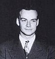
리처드 파인먼 과 마레크 카츠 (폴란드어 : Marek Kac , 영어 : Mark Kac , 1914〜1984)의 이름을 땄다.
파인먼은 이 공식을 양자역학 의 경로 적분 을 정의하기 위하여 유도하였으나, 엄밀하게 증명하지 않았다. 마레크 카츠가 이 공식의 엄밀한 증명을 1949년에 출판하였다.[ 2]
↑ Bär, Christian; Pfäffle, Frank. “Wiener measures on Riemannian manifolds and the Feynman–Kac formula” (영어). arXiv :1108.5082 . ↑ Kac, Mark (1949). “On distributions of certain Wiener functionals”. 《Transactions of the American Mathematical Society》 (영어) 65 (1): 1–13. doi :10.2307/1990512 . JSTOR 1990512 . MR 27960 .


![{\displaystyle W^{j}\colon \Omega \times [0,T]\to \mathbb {R} ^{n}}](https://wikimedia.org/api/rest_v1/media/math/render/svg/66bbfc7d9f9d9a50203747ac0a6d3d66c9f70e98)


![{\displaystyle h\colon \mathbb {R} ^{n}\times [0,T]\to \mathbb {R} }](https://wikimedia.org/api/rest_v1/media/math/render/svg/71aa7a6bf9a0d9c3f9772ab61e1ed38312319a80)
![{\displaystyle V\colon \mathbb {R} ^{n}\times [0,T]\to \mathbb {R} }](https://wikimedia.org/api/rest_v1/media/math/render/svg/21a2d87afdc7a30427324453f273adf6fdca8137)
![{\displaystyle G\colon \Omega \times [0,T]\to \mathbb {R} }](https://wikimedia.org/api/rest_v1/media/math/render/svg/d8568a2ff702887fa6b9b36c41b608ad89c248ef)


![{\displaystyle g(x,t)=\mathbb {E} \left[G(t)|X(t)=x\right]}](https://wikimedia.org/api/rest_v1/media/math/render/svg/0278c8eb5fefbff98c2333a467386bb352c27784)
![{\displaystyle g(x,T)=\mathbb {E} [f(X(T))|X(T)=x]=f(x)}](https://wikimedia.org/api/rest_v1/media/math/render/svg/7212fb0f787f85d1cbfd9170c7dcd114c17b4f32)


![{\displaystyle g(x,t)=\mathbb {E} \left[f(X(T))|X(t)=x\right]}](https://wikimedia.org/api/rest_v1/media/math/render/svg/d90fa23ec2acb284bb8e417724161e018b62c934)


![{\displaystyle {\mathcal {C}}_{x_{0}}^{0}([0,T],M)=\{f\in {\mathcal {C}}_{0}^{0}([0,T],M)\colon f(0)=x_{0}\}}](https://wikimedia.org/api/rest_v1/media/math/render/svg/8eab03c65c5ea0cb7eaf462995c8125dc86e0c86)
![{\displaystyle \operatorname {W} _{x_{0}}^{1,2}([0,T],M,g)=\left\{f\in {\mathcal {C}}_{x_{0}}^{0}([0,T],M)\colon \int _{0}^{T}g_{f(t)}({\dot {f}}(t),{\dot {f}}(t))\,\mathrm {d} t<\infty \right\}}](https://wikimedia.org/api/rest_v1/media/math/render/svg/6fe65e2d68e2147b71b4574213f3a893b63de97e)
![{\displaystyle {\mathcal {C}}_{x_{0}}^{0}([0,T],M)}](https://wikimedia.org/api/rest_v1/media/math/render/svg/ae359057c4092becfa10aca37395515de29b01a8)


![{\displaystyle {\mathcal {C}}_{x_{0},x_{T}}^{0}([0,T],M)=\{f\in {\mathcal {C}}_{0}^{0}([0,T],M)\colon f(0)=x_{0},f(T)=x_{T}\}}](https://wikimedia.org/api/rest_v1/media/math/render/svg/dda6b7ad42bd3f06c2a441fb4d43587aee1a790b)
![{\displaystyle \operatorname {W} _{x_{0},x_{T}}^{1,2}([0,T],M,g)=\operatorname {W} _{x_{0}}^{1,2}([0,T],M,g)\cap \operatorname {C} ^{0}{x_{0},x_{T}}([0,T],M)}](https://wikimedia.org/api/rest_v1/media/math/render/svg/a2a63dfd46912569779e1c4ebcdd336a6c473714)


![{\displaystyle \psi (T,x_{0})=\int _{{\mathcal {C}}_{x_{0}}^{0}([0,T],M)}\psi _{0}(x_{0})\exp \left(-\int _{0}^{T}V(f(t))\,\mathrm {d} t\right)\,\mathrm {d} W_{x_{0}}(f)}](https://wikimedia.org/api/rest_v1/media/math/render/svg/2878a0262f47aad50f316d62d74126bdcf31bfa1)


![{\displaystyle \mathbb {E} [f(X(T))\vert {\mathcal {F}}(s)]=g(X(s),s),}](https://wikimedia.org/api/rest_v1/media/math/render/svg/2d8ac45304cc8c1923443ff041d46ce67855089b)
![{\displaystyle \mathbb {E} [f(X(T))\vert {\mathcal {F}}(t)]=g(X(t),t)}](https://wikimedia.org/api/rest_v1/media/math/render/svg/e0ce5068a7a4bb37317be01ab6b8efb6fc9565f0)

![{\displaystyle {\begin{aligned}\mathbb {E} [g(X(T),t))\vert {\mathcal {F}}(s)]&=\mathbb {E} [\,\mathbb {E} [f(X(T))\vert {\mathcal {F}}(t)]\,\vert {\mathcal {F}}(s)]\\&=\mathbb {E} [f(X(T))\vert {\mathcal {F}}(s)]=g(X(s),s)\end{aligned}}}](https://wikimedia.org/api/rest_v1/media/math/render/svg/5caa953ba1cec4a3bb0fa6e7f77da5e7ddfd435b)


![{\displaystyle {\begin{aligned}\mathrm {d} g(X(t),t)&={\frac {\partial }{\partial t}}g(X(t),t)dt+{\frac {\partial }{\partial x}}g(X(t),t)dX+{\frac {1}{2}}{\frac {\partial ^{2}}{\partial x^{2}}}g(X(t),t)\mathrm {d} X\,\mathrm {d} X\\&={\frac {\partial }{\partial t}}g(X(t),t)\,\mathrm {d} t+\mu {\frac {\partial }{\partial x}}g(X(t),t)\,\mathrm {d} t+\sigma {\frac {\partial }{\partial X}}g(X(t),t)\,\mathrm {d} W(t)+{\frac {1}{2}}\sigma ^{2}{\frac {\partial ^{2}}{\partial x^{2}}}g(X(t),t)\,\mathrm {d} t\\&=\left[{\frac {\partial }{\partial t}}g(X(t),t)+\mu {\frac {\partial }{\partial x}}g(X(t),t)+{\frac {1}{2}}\sigma ^{2}{\frac {\partial ^{2}}{\partial x^{2}}}g(X(t),t)\right]\,\mathrm {d} t+\sigma {\frac {\partial }{\partial x}}g(X(t),t)\,\mathrm {d} W(t)\end{aligned}}}](https://wikimedia.org/api/rest_v1/media/math/render/svg/2a7ee134b16145165787be5354ad15742fc83a26)


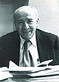 마레크 카츠
